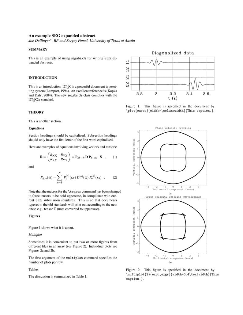
Template for SEG abstract
Author:
Sergey Fomel
Last Updated:
před 5 lety
License:
LaTeX Project Public License 1.3c
Abstract:
Template for writing SEG abstract.

\begin
Discover why over 25 million people worldwide trust Overleaf with their work.
Template for writing SEG abstract.

\begin
Discover why over 25 million people worldwide trust Overleaf with their work.
\documentclass{segabs}

% An example of defining macros
\newcommand{\rs}[1]{\mathstrut\mbox{\scriptsize\rm #1}}
\newcommand{\rr}[1]{\mbox{\rm #1}}

\begin{document}

\title{An example SEG expanded abstract}

\renewcommand{\thefootnote}{\fnsymbol{footnote}}

\author{Joe Dellinger\footnotemark[1], BP
  and Sergey Fomel, University of Texas at Austin}

\footer{Example}
\lefthead{Dellinger \& Fomel}
\righthead{SEG abstract example}

\maketitle

\begin{abstract}
  This is an example of using \textsf{segabs.cls} for writing
  SEG expanded abstracts.
\end{abstract}

\section{Introduction}

This is an introduction. \LaTeX\ is a powerful document typesetting
system \cite[]{lamport}. An excellent reference is \cite[]{kopka}. The
new \textsf{segabs.cls} class complies with the \LaTeX2e\ standard.

\section*{Theory}

This is another section.

\subsection{Equations}

Section headings should be capitalized. Subsection headings should
only have the first letter of the first word capitalized.

Here are examples of equations involving vectors and tensors:
\begin{equation}
\tensor{R} =
\pmatrix{R_{\rs{XX}} & R_{\rs{YX}} \cr R_{\rs{XY}} & R_{\rs{YY}}}
=
\tensor{P}_{M\rightarrow R} \; \tensor{D} \; \tensor{P}_{S\rightarrow M}
\;\;\; \tensor{S} \ \ \  ,
\label{SVD}
\end{equation}
and
\begin{equation}
R_{j,m}(\omega) =
\sum_{n=1}^{N} \, \,
P_{j}^{(n)}(\mathbf{x}_R) \, \,
D^{(n)}(\omega) \, \,
P_{m}^{(n)}(\mathbf{x}_S) \ \ \ .
\label{SVDray}
\end{equation}

Note that the macros for the \verb#\tensor# command has been changed
to force tensors to be bold uppercase, in compliance with current SEG
submission standards. This is so that documents typeset to the old
standards will print out according to the new ones: e.g., tensor
$\tensor{t}$ (note converted to uppercase).

\subsection*{Figures}
\renewcommand{\figdir}{Fig} % figure directory

Figure~\ref{fig:waves} shows what it is about.

\plot{waves}{width=\columnwidth}
{This figure is specified in the document by \texttt{
    $\backslash$plot\{waves\}\{width=$\backslash$columnwidth\}\{This caption.\}}.
}

\subsubsection{Multiplot}

Sometimes it is convenient to put two or
more figures from different files in an array (see
Figure~\ref{fig:exph,exgr}). Individual plots are
Figures~\ref{fig:exph} and~\ref{fig:exgr}.

\multiplot{2}{exph,exgr}{width=0.4\textwidth}
{This figure is specified in the document by \texttt{
    $\backslash$multiplot\{2\}\{exph,exgr\}\{width=0.4$\backslash$textwidth\}\{This caption.\}}.
}

The first argument of the \texttt{multiplot} command specifies the
number of plots per row.

\subsection{Tables}

The discussion is summarized in Table~\ref{tbl:example}.

\tabl{example}{This table is specified in the document by \texttt{
    $\backslash$tabl\{example\}\{This caption.\}\{\ldots\}}.
}{
  \begin{center}
    \begin{tabular}{|c|c|c|}
      \hline
      \multicolumn{3}{|c|}{Table Example} \\
      \hline
      migration\rule[-2ex]{0ex}{5ex} &
      $\omega \rightarrow k_z$ &
      $k_y^2+k-z^2\cos^2 \psi=4\omega^2/v^2$ \\
      \hline
      \parbox{1in}{zero-offset\\diffraction}\rule[-4ex]{0ex}{8ex} &
      $k_z\rightarrow\omega_0$ &
      $k_y^2+k_z^2=4\omega_0^2/v^2$ \\
      \hline
      DMO+NMO\rule[-2ex]{0in}{5ex} & $\omega\rightarrow\omega_0$ &
      $\frac{1}{4}
      v^2k_y^2\sin^2\psi+\omega_0^2\cos^2\psi=\omega^2$ \\
      \hline
      radial DMO\rule[-2ex]{0in}{5ex} & $\omega\rightarrow\omega_s$ &
      $\frac{1}{4}v^2k_y^2\sin^2\psi+\omega_s^2=\omega^2$\\
      \hline
      radial NMO\rule[-2ex]{0in}{5ex} & $\omega_s\rightarrow\omega_0$ &
      $\omega_0\cos\psi=\omega_s$\\
      \hline
    \end{tabular}
  \end{center}
}

\section{ACKNOWLEDGMENTS}

I wish to thank Ivan P\v{s}en\v{c}\'{\i}k and Fr\'ed\'eric Billette
for having names with non-English letters in them.  I wish to thank
\cite{Cerveny} for providing an example of how to make a bib file that
includes an author whose name begins with a non-English character and
\cite{forgues96} for providing both an example of referencing a Ph.D.
thesis and yet more non-English characters.

\append{Appendix example}

According to the new SEG standard, appendices come before references.

\begin{equation}
\frac{\partial U}{\partial z} =
\left\{
  \sqrt{\frac{1}{v^2} - \left[\frac{\partial t}{\partial g}\right]^2} +
  \sqrt{\frac{1}{v^2} - \left[\frac{\partial t}{\partial s}\right]^2}
\right\}
\frac{\partial U}{\partial t}
\label{eqn:partial}
\end{equation}
It is important to get equation~\ref{eqn:partial} right.

\append{Another appendix}

\begin{equation}
\frac{\partial U}{\partial z} =
\left\{
  \sqrt{\frac{1}{v^2} - \left[\frac{\partial t}{\partial g}\right]^2} +
  \sqrt{\frac{1}{v^2} - \left[\frac{\partial t}{\partial s}\right]^2}
\right\}
\frac{\partial U}{\partial t}
\label{eqn:partial2}
\end{equation}
Too lazy to type a different equation but note the numeration.

The error comparison is provided in Figure~\ref{fig:errgrp}.

\plot*{errgrp}{width=0.8\textwidth} {This figure is specified in the
  document by \texttt{
    $\backslash$plot*\{errgrp\}\{width=0.8$\backslash$textwidth\}\{This caption.\}}.  }

\onecolumn

\append{The source of the bibliography}
\verbatiminput{example.bib}

\twocolumn

\bibliographystyle{seg}  % style file is seg.bst
\bibliography{example}

\end{document}